How to Use the VLOOKUP Function in Excel

Before we dive into the universe of VLOOKUP, let's understand what Excel is. Microsoft Excel is a spreadsheet software and part of the Microsoft Office suite, used in corporate and academic settings for the manipulation, analysis, and visualization of data.

With its powerful calculation tools, charts, pivot tables, and functions like VLOOKUP, it has become an indispensable tool for professionals from various fields. In this post, we will explore how to perform VLOOKUP in Excel, a crucial skill for those who wish to maximize this tool.

Understanding VLOOKUP

VLOOKUP is a function in Excel that allows you to search for a value in one column and return a corresponding value from another column in the same row. This function is extremely useful for comparing and extracting data from large tables, becoming a valuable skill for any Excel user.

Preparing Your Data:

To use VLOOKUP effectively, it is crucial that your data is well organized. The lookup key, that is, the value you want to find, should be in the first column of the selected range, with related data in subsequent columns.

The Syntax of VLOOKUP:

The VLOOKUP function follows the following order:

=VLOOKUP(lookup_value, table_array, col_index_num, [range_lookup])

Each part of this syntax plays a specific role:
lookup_value: The value you want to search for.
table_array: Where Excel should look for the value.
col_index_num: The column number that contains the value to be returned.
range_lookup: Defines whether the search will be for an exact match or an approximate match.

Example 1: Search

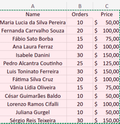
Consider the following scenario: a confectionery that has a table with the names of its customers, the number of orders, and the value received for the products, as shown in the image below, and wishes to find the value for the customer Isabele Danini.

Notice that the column "Name" is the "lookup_value," while "table_array" refers to the entire table range.

The variable "col_index_num" represents the column where the desired information will be searched. Here, we are looking for the value spent by Isabele, which corresponds to the third column of the table. Therefore, the value of "col_index_num" is 3.

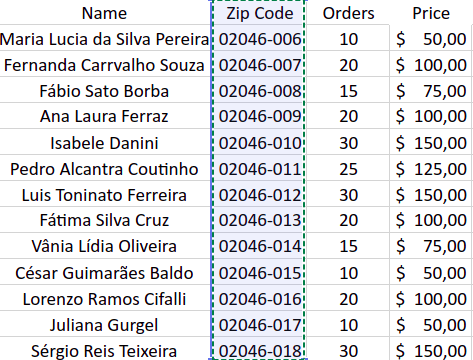
If there were another column before the "Orders" column, for example, with the customers' ZIP codes, and it was selected in our "table_array" range, then the "col_index_num" would become 4.

In "[range_lookup]," we will put 0 (FALSE), so the function will have an exact match. The TRUE option allows an approximate match.

To find the value of Isabele's orders, we are going to use the formula:

Here, "Isabele Danini" is the lookup value, "A1:C14" is what was selected and where Excel will search, "3" is the sales value column, and 0 ("FALSE") specifies that we want an exact match.

Example 2: Table Comparison

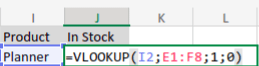
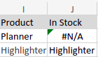
In this example, we use the case of an online stationery store that sells a variety of products. To maintain organization, they use two separate tables: one displaying products available for sale and another showing items in stock, as illustrated in the following image.

Now, let's check if the planner is in stock. For this, we use the VLOOKUP function selecting the table related to products in stock.

Note that the "col_index_num" function is 1 because the information sought is in the first column.

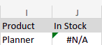
As the product is not in stock, the function returns #N/A.

While in comparison, the product "Highlighter" is in stock, so it was its own name.

Example 3: Multiple Conditions

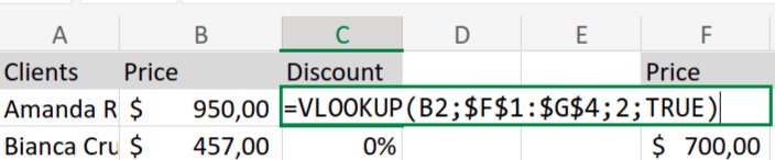
In this example, we have a beauty salon with the following policy: customers who spend more than $700.00 on purchases will receive a 30% discount, and those spending more than $900.00 will receive a 40% discount.

A table was created with the ranges of values and their discounts.

Now, we will use the VLOOKUP function. Note that, in this case, the "table_array" is the second table, with the values and discounts of the salon. As we will use this table for all customers, we add the $ symbol to not change the cell, as seen in the image below.

Also note that, in this case, we use the "range_lookup" TRUE, which can be represented by the number 1.

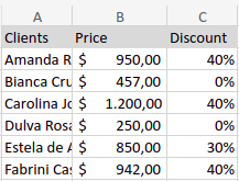
Dragging down, we have discounts for all customers.

Why Not Use the IF Function?

The IF function is well known and more appropriate for situations where there are only one or two conditions, that is, simpler cases.

In Example 3, the IF function would be much larger and take much more time, whereas the VLOOKUP function is more agile and simpler in this case. It is necessary to consider the amount of data and its conditions to determine which function is better for solving your problem.

Centralizing Data in Excel

Enhance your Excel analysis with the VLOOKUP function and take your data management to a new level. With Kondado, it's possible to centralize data from over 80 sources directly into Excel, a new destination for your data analysis. If you wish to centralize your data automatically and efficiently, count on Kondado. Try our platform for free, without the need for a credit card, by clicking here. Transform your way of working with data today!

Tips and Precautions:

The search key must always be in the first column of the range.
VLOOKUP can differentiate between uppercase and lowercase in some versions of Excel.
If the function returns #N/A, it means that the searched value is not present in the range.

Conclusion

Mastering VLOOKUP in Excel is a fundamental step for those who want efficiency and precision in data manipulation. This function, although simple, can bring great benefits in terms of time saved and increased productivity.